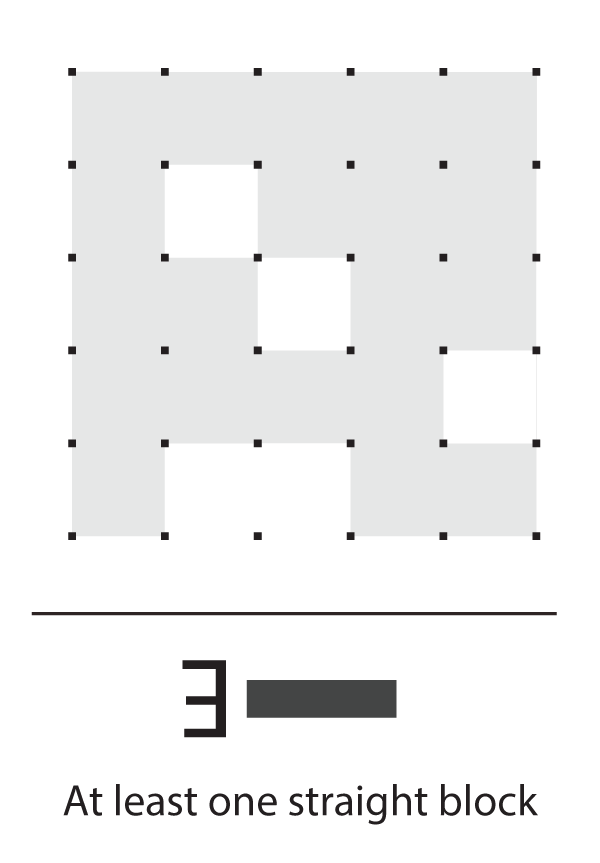
The following shape is comprised of exactly five tetrominoes, shown in light gray. The borders between them, however, are not shown. Your job is to draw borders between the dots such that the tetrominoes are visible. Can you do it?

It’s a trick question: there is no unique solution. Here are the four solutions:


This particular puzzle is fairly easy, since it’s clear that there must be an I-block on the left. This is a form of forward-checking, and it’s something experienced puzzle solvers do all the time: they can eliminate fruitless search paths before spending any time on them. Even so, some tougher puzzles require you to backtrack: the hardest Sudoku puzzles may need multiple layers of recursion before a particular partial solution is identified as inconsistent.
Even if getting all solutions to a puzzle is easy, logic puzzles need to have a single solution. If not, solving them is bound to be a very frustrating experience, especially for more complex puzzles. How, then, can we come up with a puzzle based on the idea of tiling an orthogonal polygon with tetrominoes if such simple shapes have so many tilings? The answer is to impose a global constraint: for instance, if we require that there are no T-blocks, the only solution is the top-left one. So, how can we get all possible solutions to such a puzzle, such that we can come up with a constraint that enforces a single solution?
Constraint propagation
Constraint satisfaction problems (CSPs) are a very broad class of combinatorial problems. Logic puzzles such as Sudoku, Nonograms, Shikaku, Hitori, Hashi, and Nurikabe, to name a few, are all examples of CSPs, and so is the little tetromino puzzle above. Constraint satisfaction problems can be recast as SAT problems (Boolean satisfiability problems), but the geometrical nature of the tetromino puzzle means that expressing it as a SAT problem is not easy. Instead, let’s take advantage of the vast machinery of graph theory and express the puzzle above as a graph, where the 1×1 blocks correspond to vertices, and their shared edges correspond to edges.
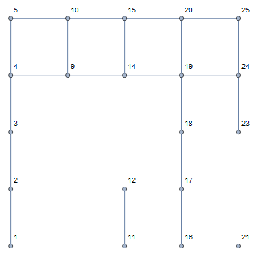
This graph was reproduced in Mathematica, which features a powerful set of tools for graph theory visualisation. All we have to do now is delete enough edges, and a solution will reveal itself once the graph is composed of exactly 5 disconnected subgraphs with 4 vertices each. We could try to brute-force the problem, but that’s a recipe for disaster: checking all 2^25 possible states is not something that we want to do.
What, then, should we do? Here is where constraint propagation comes to the rescue. Instead of iterating over the vast state space, we will perform a breadth-first search, where the depth corresponds to how many edges we have removed from the graph. Thus, the decision tree is made up of nodes, each of which is a 25-bit binary number (since there are 25 edges to be deleted). A 1 corresponds to an edge which is still there, whereas a 0 corresponds to a removed edge.
The method we use is a simple version of arc consistency. At each node, we have already cut some edges (0s), and make further cuts (i.e. split the node into children, each of which turns a different 1 into 0). Then, we only propagate down the branch where the new cut will lead to a consistent solution: this is a simple implementation of backtracking (this may produce some double counting of states, which can be easily taken care of using the inbuilt RemoveDuplicates function).
And what is the consistency check we use? It’s very simple: given enough edge cuts, the graph will eventually become disconnected. The consistency check is therefore that all disconnected subgraphs have 4n vertices. Any partial solution that doesn’t satisfy this constraint will never satisfy it even if more edges are removed, and no further search is performed down that branch.
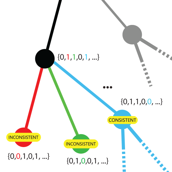
Forward checking/full look ahead (which take into account consistency between uninstanced variables) are generally faster, since they rule out bigger chunks of the search space. The difference is easily seen in the 8-queens problem: instead of adding queens to the board and checking whether they are in line of sight of another queen, we only place further queens not in a row, column, or diagonal of another queen. Applying such a constraint is slightly more challenging here, since it’s not much more algorithmically efficient to rule out child nodes (as opposed to checking them for consistency).
Running this algorithm returns more graphs than there are unique solutions. This is because some resulting graphs are equivalent up to relabellings within their disconnected components. Sorting the disconnected components of all the graphs in canonical order ensures that graphs whose disconnected components are relabellings of each others coincide, and so using the RemoveDuplicates function again produces all possible solutions:
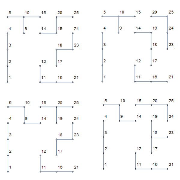
Graph partitioning is a very exciting field (especially since graph partitioning is NP-hard, even subject to balancing constraints), and there are of course much more sophisticated algorithms than the one presented here. Even so, it’s quite interesting to see what kinds of puzzles can be generated and tested with the help of a simple algorithm.
A few more puzzles
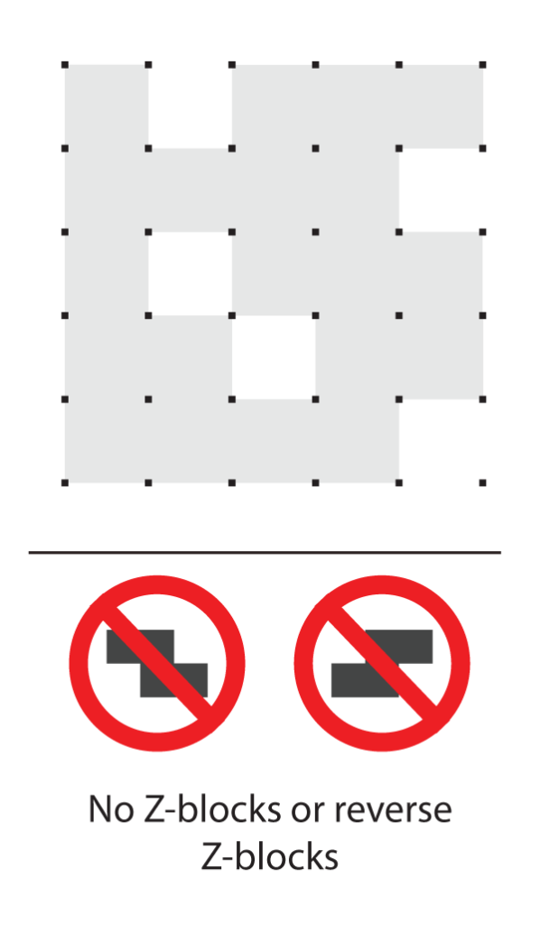
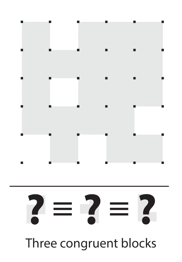
I leave you with a few puzzles of the same variety – and this time, they do have a unique solution, honest. Can you solve them?
